For ACT Students
The ACT is a timed exam...60 questions for 60 minutes
This implies that you have to solve each question in one minute.
Some questions will typically take less than a minute a solve.
Some questions will typically take more than a minute to solve.
The goal is to maximize your time. You use the time saved on those questions you
solved in less than a minute, to solve the questions that will take more than a minute.
So, you should try to solve each question correctly and timely.
So, it is not just solving a question correctly, but solving it correctly on time.
Please ensure you attempt all ACT questions.
There is no negative penalty for any wrong answer.
For SAT Students
Any question labeled SAT-C is a question that allows a calculator.
Any question labeled SAT-NC is a question that does not allow a calculator.
For JAMB Students
Calculators are not allowed. So, the questions are solved in a way that does not require a calculator.
For WASSCE Students
Any question labeled WASCCE is a question for the WASCCE General Mathematics
Any question labeled WASSCE-FM is a question for the WASSCE Further Mathematics/Elective Mathematics
For NSC Students For the Questions:
Any space included in a number indicates a comma used to separate digits...separating multiples of three digits
from behind.
Any comma included in a number indicates a decimal point. For the Solutions:
Decimals are used appropriately rather than commas
Commas are used to separate digits appropriately.
Notatable Notes About Mean and Standard Deviation.
(1.) Given an initial dataset:
If the value of a variable is decreased, the total sum of the frequencies and the values of the variable,
Σfx of the new dataset will decrease, hence the mean and the standard deviation of the new dataset
will decrease.
The mean and the standard deviation will decrease.
(2.) Given an initial dataset:
If a new value, lower than the minimum value of the initial dataset is included in it:
The mean will decrease and the standard deviation will increase.
(3.) Given an initial dataset:
If a new value, higher than the maximum value of the initial dataset is included in it:
The mean will increase and the standard deviation will decrease.
Solve all questions.
Show all work.
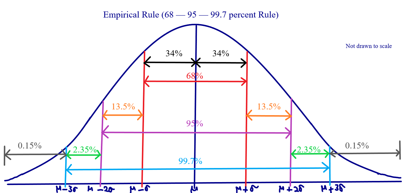
The Empirical Rule
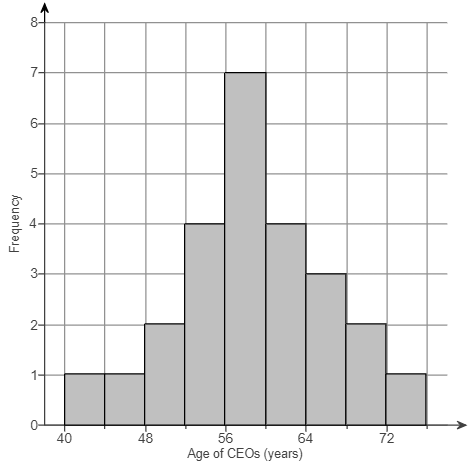
(1.) The histogram shows the ages of 25 CEOs listed on a certain website.
Based on the distribution, what is the approximate mean age of the CEOs in this data set?
Write a sentence in context (using words in the question) interpreting the estimated mean.
The distribution is symmetric, so the typical value, known as the mean, is located in the center
of the histogram.
The typical CEO is between 56 and 60 years.
(2.) GCSE The tibia is the bone that connects the knee to the ankle bone.
The lengths of the tibia bones in modern-day adult makes have a normal distribution with mean
36.0 cm and
standard deviation 2.8 cm Almost all adult male tibia bones have lengths that are between a cm and b cm
Calculate the values of a and b
Empirical Rule: 68 - 95 - 99.7% Rule
Part of the Empirical Rule states that 99.7% of the adult male tibia bones have lengths within
(below and above) 3 standard
deviations from the mean
$
\mu = 36.0\; cm \\[3ex]
\sigma = 2.8\;cm \\[3ex]
3\sigma = 3(2.8) = 8.4\;cm \\[3ex]
\underline{3\;standard\;\;deviations\;\;below\;\;the\;\;mean} \\[3ex]
\mu - 3\sigma \\[3ex]
36 - 8.4 \\[3ex]
27.6 \\[3ex]
a = 27.6\;cm \\[3ex]
\underline{3\;standard\;\;deviations\;\;above\;\;the\;\;mean} \\[3ex]
\mu + 3\sigma \\[3ex]
36 + 8.4 \\[3ex]
44.4 \\[3ex]
b = 44.4\;cm \\[3ex]
$
About 99.7% of adult male tibia bones have lengths between 27.6 cm and 44.4 cm
(3.) The prices (in $ thousands) of a sample of three-bedroom homes for sale in State A and State B
are shown in the table below.
State A
State B
291
192
336
211
129
414
182
130
115
197
172
291
180
127
(I.) In a few sentences, compare the prices of these homes.
(II.) Answer the questions of which state had the most expensive homes and which had the most
variability in home prices.
$
\underline{State\;A} \\[3ex]
(a.) \\[3ex]
mean = \bar{x} = \dfrac{\Sigma fx}{\Sigma f} \\[5ex]
= \dfrac{1562}{7} \\[5ex]
= 223.1428571 \\[3ex]
\approx 223.14...rounded\;\;to\;\;the\;\;nearest\;\;hundredth \\[5ex]
(b.) \\[3ex]
variance = s^2 = \dfrac{\Sigma f(x - \bar{x})^2}{\Sigma f - 1} \\[5ex]
= \dfrac{60750.85714}{7 - 1} \\[5ex]
= \dfrac{60750.85714}{6} \\[5ex]
= 10125.14286 \\[3ex]
standard\;\;deviation = s = \sqrt{s^2} \\[3ex]
= \sqrt{10125.14286} \\[3ex]
= 100.6237688 \\[3ex]
\approx 100.62...rounded\;\;to\;\;the\;\;nearest\;\;hundredth \\[3ex]
$
(I.) This implies that:
The typical price (in $ thousands) for a three-bedroom home in State A is $200.71
The typical price (in $ thousands) for a three-bedroom home in State B is $223.14
Therefore, the typical price for a three-bedroom home is higher in State B.
The standard deviation of price (in $ thousands) for a three-bedroom home in State A
is $82.21
The standard deviation of price (in $ thousands) for a three-bedroom home in State B
is $100.62
Therefore, the standard deviation of price for a three-bedroom home is higher in State B.
(II.) Therefore, the prices for three-bedroom homes tend to be lower and have less variation in
State A than in State B.
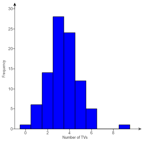
(4.) The histogram shows the number of televisions in the homes of 90 community college students.
Judging from the histogram, what is the approximate mean number of televisions in the homes in this
collection? Explain.
The mean number of televisions per home is between 3 and 4.
The mean is near the center, which is due to the fact that the histogram is roughly symmetric.
(5.) The table shows the lengths (in miles) of major rivers in North America.
River
Length (in miles)
Colorado
1450
Mackenzie
2635
Mississippi-Missouri-Red Rock
3710
Rio Grande
1900
Yukon
1979
(a.) Determine and interpret (report in context) the mean.
(b.) Determine the standard deviation.
(c.) Which river contributes most to the size of the standard deviation?
(d.) If the St. Lawrence River (length 800 miles) were included in the data set, explain how the mean
and standard deviation from parts (a) and (b) would be affected?
(e.) Recalculate the mean and the standard deviation including the St. Lawrence River.
Length, $x$
$f$
$fx$
$x - \bar{x}$
$(x - \bar{x})^2$
$f(x - \bar{x})^2$
$1450$
$1$
$1450$
$-884.8$
$782871.04$
$782871.04$
$2635$
$1$
$2635$
$300.2$
$90120.04$
$90120.04$
$3710$
$1$
$3710$
$1375.2$
$1891175.04$
$1891175.04$
$1900$
$1$
$1900$
$-434.8$
$189051.04$
$189051.04$
$1979$
$1$
$1979$
$-355.8$
$126593.64$
$126593.64$
$\Sigma f = 5$
$\Sigma fx = 11674$
$\Sigma f(x - \bar{x})^2 = 15286.8$
$
(a.) \\[3ex]
mean = \bar{x} = \dfrac{\Sigma fx}{\Sigma f} \\[5ex]
= \dfrac{11674}{5} \\[5ex]
= 2334.8 \\[3ex]
$
The mean length of the major rivers in North America is approximately 2335 miles (rounded to the
nearest integer).
$
(b.) \\[3ex]
variance = s^2 = \dfrac{\Sigma f(x - \bar{x})^2}{\Sigma f - 1} \\[5ex]
= \dfrac{3079810.8}{5 - 1} \\[5ex]
= \dfrac{3079810.8}{4} \\[5ex]
= 769952.7 \\[3ex]
standard\;\;deviation = s = \sqrt{s^2} \\[3ex]
= \sqrt{769952.7} \\[3ex]
= 877.4694866 \\[3ex]
$
The standard deviation is approximately 877 miles. (value is rounded to the nearest integer)
(c.) Mississippi-Missouri-Red Rock River contributes most to the size of the standard deviation
because it is the furthest from the mean.
(d.) Given an initial dataset:
If a new value, lower than the minimum value of the initial dataset is added to it:
The mean will decrease and the standard deviation will increase.
$
(e.) \\[3ex]
n = 6 \\[3ex]
mean = \bar{x} = \dfrac{\Sigma fx}{\Sigma f} \\[5ex]
= \dfrac{12474}{6} \\[5ex]
= 2079 \\[3ex]
$
The new mean is 2079 miles.
$
(b.) \\[3ex]
variance = s^2 = \dfrac{\Sigma f(x - \bar{x})^2}{\Sigma f - 1} \\[5ex]
= \dfrac{5042820}{6 - 1} \\[5ex]
= \dfrac{5042820}{5} \\[5ex]
= 1008564 \\[3ex]
standard\;\;deviation = s = \sqrt{s^2} \\[3ex]
= \sqrt{1008564} \\[3ex]
= 1004.272871 \\[3ex]
$
The standard deviation is approximately 1004 miles. (value is rounded to the nearest integer)
(6.) The table shows the location and number of floors in some of the tallest buildings in the world.
City
Number of Floors
City 1
164
City 2
123
City 3
114
City 4
102
City 5
102
(a.) Determine and interpret (report in context) the mean number of floors in this data set.
(b.) Determine and interpret the standard deviation of the number of floors in this data set.
(c.) Which of the given observations is farthest from the mean and therefore contributes most to the
standard deviation?
$
(a.) \\[3ex]
n = 5 \\[3ex]
Mean = \bar{x} = \dfrac{\Sigma Floors}{n} \\[5ex]
= \dfrac{164 + 123 + 114 + 102 + 102}{5} \\[5ex]
= \dfrac{605}{5} \\[5ex]
= 121 \\[3ex]
$
The typical number of floors of the tallest buildings is 121 floors.
(b.)
Floor, $x$
$f$
$fx$
$x - \bar{x}$
$(x - \bar{x})^2$
$f(x - \bar{x})^2$
$164$
$1$
$164$
$43$
$1849$
$1849$
$123$
$1$
$123$
$2$
$4$
$4$
$114$
$1$
$114$
$-7$
$49$
$49$
$102$
$2$
$204$
$-19$
$361$
$722$
$\Sigma f = 5$
$\Sigma f(x - \bar{x})^2 = 2624$
$
variance = s^2 = \dfrac{\Sigma f(x - \bar{x})^2}{\Sigma f - 1} \\[5ex]
= \dfrac{2624}{5 - 1} \\[5ex]
= \dfrac{2624}{4} \\[5ex]
= 656 \\[3ex]
standard\;\;deviation = s = \sqrt{s^2} \\[3ex]
= \sqrt{656} \\[3ex]
= 25.61249695 \\[3ex]
$
The standard deviation of the number of floors of the tallest buildings is approximately 25.6 floors
(value is rounded to one decimal place).
(c.) The number farthest from the mean that contributes the most to the given standard deviation is
164, which represents the number of floors in City 1.
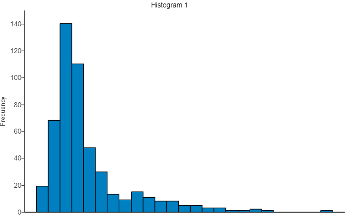
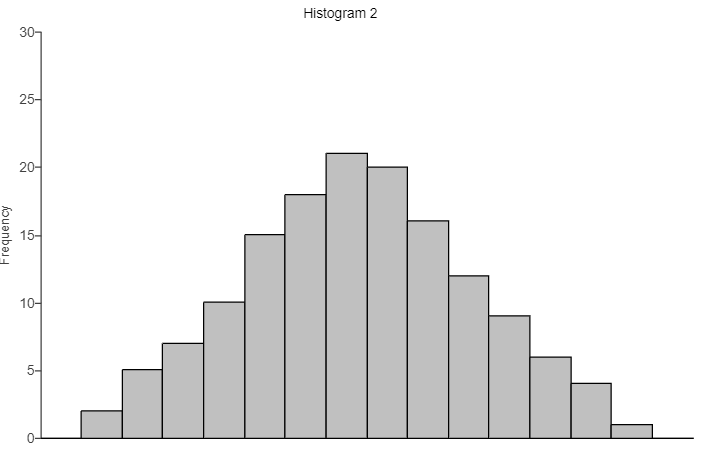
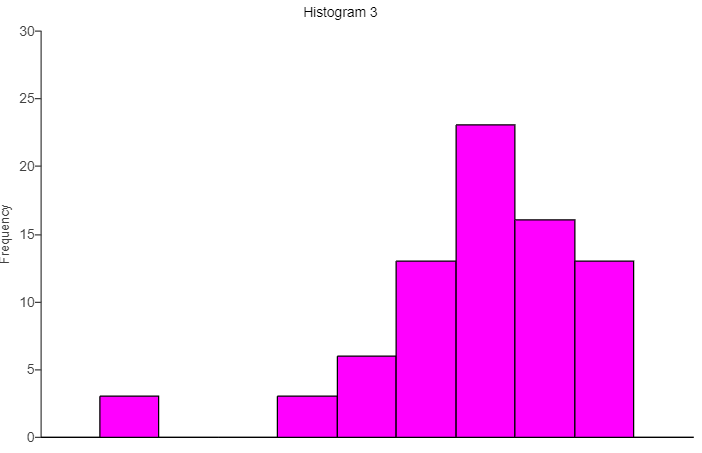
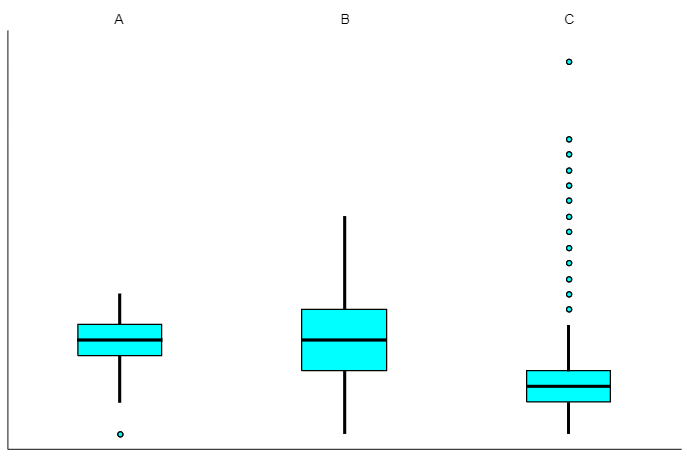
(7.) Three histograms and three boxplots are given below.
(a.) Report the shape of each histogram.
(b.) Match each histogram with the corresponding boxplot (A, B, or C)
(a.) Histogram 1 shows a right-skewed distribution.
Histogram 2 shows a symmetric distribution.
Histogram 3 shows a left-skewed distribution.
(b.) Boxplot A corresponds to Histogram 3
Boxplot B corresponds to Histogram 2
Boxplot C corresponds to Histogram 1
(8.) GCSE [Continued from Question (2.)]
The lengths of tibia bones in modern-day adult females have a normal distribution with
mean 33.8 cm
and standard deviation 2.2 cm
(a.) A tibia bone is discovered measuring 34.5 cm
Alice says the bone is more likely to be from an adult female than an adult male.
Evaluate Alice's statement.
$
Use\;\;standardized\;\;score = \dfrac{value - mean}{standard\;\;deviation} \\[5ex]
$
(b.) In fact, the bone in part(a.) was discovered on an old Roman site and is estimated as being
about 1900 years old.
Is the conclusion made in part(a.) likely to be valid?
Explain your answer.
The question wants us to evaluate Alice's statement using the z-score formula
$
(a.) \\[3ex]
\underline{Adult\;\;Female} \\[3ex]
\mu = 33.8\;cm \\[3ex]
\sigma = 2.2\;cm \\[3ex]
x = 34.5 \\[3ex]
z = \dfrac{x - \mu}{\sigma} \\[5ex]
z = \dfrac{34.5 - 33.8}{2.2} \\[5ex]
z = \dfrac{0.7}{2.2} \\[5ex]
z = 0.3181818182 \approx 0.32 \\[5ex]
\underline{Adult\;\;Male} \\[3ex]
\mu = 36\;cm \\[3ex]
\sigma = 2.8\;cm \\[3ex]
x = 34.5 \\[3ex]
z = \dfrac{x - \mu}{\sigma} \\[5ex]
z = \dfrac{34.5 - 36}{2.8} \\[5ex]
z = -\dfrac{1.5}{2.8} \\[5ex]
z = -0.5357142857 \approx -0.54 \\[3ex]
$
(b.)
A data value is usual if $-2.00 \lt z-score \lt 2.00$
A data value is unusual if $z-score \lt -2.00$ or if $z-score \gt 2.00$
Adult Female: Because $-2 \lt 0.32 \lt 2$; the data value is usual
Adult Male: Because $-2 \lt -0.54 \lt 2$; the data value is also usual
Both data values are usual.
Hence, there is insufficient evidence to verify Alice' statement.
However,
Because of the positive z-score for the adult female
(a positive z-score indicates that the data value is above the mean), the bone may likely be
from an adult female than
from an adult male.
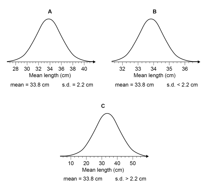
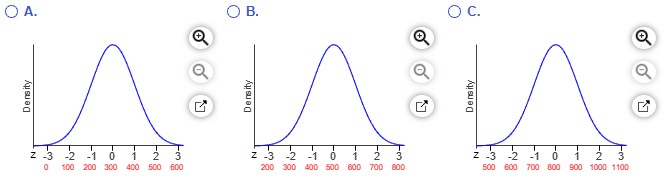
(9.) GCSE [Continued from Questions (2.) and (8.)]
A number of samples of tibia length for modern-day adult females were collected.
The histogram is drawn to represent the mean values of these samples.
Which normal distribution curve should the histogram most look like?
Empirical Rule: 68 - 95 - 99.7% Rule
Part of the Empirical Rule states that 99.7% of the adult male tibia bones have lengths within
(below and above) 3
standard
deviations from the mean
$
\mu = 33.8\; cm \\[3ex]
\sigma = 2.2\;cm \\[3ex]
3\sigma = 3(2.2) = 6.6\;cm \\[3ex]
\underline{3\;standard\;\;deviations\;\;below\;\;the\;\;mean} \\[3ex]
\mu - 3\sigma \\[3ex]
33.8 - 6.6 \\[3ex]
= 27.2\;cm \\[3ex]
\underline{3\;standard\;\;deviations\;\;above\;\;the\;\;mean} \\[3ex]
\mu + 3\sigma \\[3ex]
33.8 + 6.6 \\[3ex]
= 40.4\;cm \\[3ex]
$
About 99.7% of adult female tibia bones have lengths between 27.2 cm and 40.4 cm
The option that matches this result is Option (A.)
(10.) Babies born after 40 weeks gestation have a mean length of 52.6 centimeters (about 20.7 inches).
Babies born one month early have a mean length of 46.4 cm.
Assume both standard deviations are 2.7 cm and the distributions and unimodal and symmetric.
(a.) Find the standardized score (z-score), relative to babies born after 40 weeks gestation, for a
baby with a birth length of 45 cm.
(b.) Find the standardized score for a birth length of 45 cm for a child born one month early, using
46.4 as the mean.
(c.) For which group is a birth length of 45 cm more common?
Explain what that means. Unusual z-scores are far from 0.
$
z = \dfrac{x - \mu}{\sigma} \\[5ex]
\underline{Born\;\;after\;\;40\;\;weeks\;\;gestation} \\[3ex]
\mu = 52.6\;cm \\[3ex]
\sigma = 2.7\;cm \\[3ex]
(a.) \\[3ex]
x = 45\;cm \\[3ex]
z = \dfrac{45 - 52.6}{2.7} \\[5ex]
z = -2.814814815 \\[3ex]
z \approx -2.81 \\[5ex]
(b.) \\[3ex]
\underline{Born\;\;one\;\;month\;\;early} \\[3ex]
\mu = 46.4\;cm \\[3ex]
\sigma = 2.7\;cm \\[3ex]
x = 45\;cm \\[3ex]
z = \dfrac{45 - 46.4}{2.7} \\[5ex]
z = -0.5185185185 \\[3ex]
z \approx -0.52 \\[3ex]
$
(c.) −0.52 is closer to 0 than −2.81
−2.81 is far from 0, hence it is unusual.
A birth length of 45 cm is more common for babies born one month early.
This makes sense because babies grow during gestation, and babies born one month early have had
less time to grow.
(11.) The table shows the heights of some of the tallest roller coasters in a certain area.
Roller Coaster
Height (in feet)
Roller Coaster 1
443
Roller Coaster 2
428
Roller Coaster 3
417
Roller Coaster 4
332
Roller Coaster 5
306
(a.) Determine and interpret (report in context) the mean height of these roller coasters.
(b.) Determine and interpret the standard deviation of the height of these roller coasters.
(c.) If roller coaster 1 was only 428 feet high, how would this affect the mean and standard deviation
you calculated in (a) and (b)?
(d.) Recalculate the mean and standard deviation using 428 feet as the height of roller coaster 1.
Floor, $x$
$f$
$fx$
$x - \bar{x}$
$(x - \bar{x})^2$
$f(x - \bar{x})^2$
$443$
$1$
$443$
$57.8$
$3340.84$
$3340.84$
$428$
$1$
$428$
$42.8$
$1831.84$
$1831.84$
$417$
$1$
$417$
$31.8$
$1011.24$
$1011.24$
$332$
$1$
$332$
$-53.2$
$2830.24$
$2830.24$
$306$
$1$
$306$
$-79.2$
$6272.64$
$6272.64$
$\Sigma f = 5$
$\Sigma fx = 1926$
$\Sigma f(x - \bar{x})^2 = 15286.8$
$
(a.) \\[3ex]
mean = \bar{x} = \dfrac{\Sigma fx}{\Sigma f} \\[5ex]
= \dfrac{1926}{5} \\[5ex]
= 385.2 \\[3ex]
$
The typical height of the tallest roller coasters in this area is 385.2 feet.
$
(b.) \\[3ex]
variance = s^2 = \dfrac{\Sigma f(x - \bar{x})^2}{\Sigma f - 1} \\[5ex]
= \dfrac{15286.8}{5 - 1} \\[5ex]
= \dfrac{15286.8}{4} \\[5ex]
= 3821.7 \\[3ex]
standard\;\;deviation = s = \sqrt{s^2} \\[3ex]
= \sqrt{3821.7} \\[3ex]
= 61.81989971 \\[3ex]
$
The standard deviation of the height of the tallest roller coasters in this area is approximately
61.8 feet. (value is rounded to 1 decimal place)
(c.) Given an initial dataset:
If the value of a variable is decreased, the total sum of the frequencies and the values of the
variable, Σfx of the new dataset will decrease, hence the mean and the standard
deviation of the new dataset will decrease.
The mean and standard deviation will decrease.
Floor, $x$
$f$
$fx$
$x - \bar{x}$
$(x - \bar{x})^2$
$f(x - \bar{x})^2$
$428$
$1$
$428$
$45.8$
$2097.64$
$2097.64$
$428$
$1$
$428$
$45.8$
$2097.64$
$2097.64$
$417$
$1$
$417$
$34.8$
$1211.04$
$1211.04$
$332$
$1$
$332$
$-50.2$
$2520.04$
$2520.04$
$306$
$1$
$306$
$-76.2$
$5806.44$
$5806.44$
$\Sigma f = 5$
$\Sigma fx = 1911$
$\Sigma f(x - \bar{x})^2 = 13732.8$
$
mean = \bar{x} = \dfrac{\Sigma fx}{\Sigma f} \\[5ex]
= \dfrac{1911}{5} \\[5ex]
= 382.2 \\[3ex]
$
The new mean is 382.2 feet.
$
variance = s^2 = \dfrac{\Sigma f(x - \bar{x})^2}{\Sigma f - 1} \\[5ex]
= \dfrac{13732.8}{5 - 1} \\[5ex]
= \dfrac{13732.8}{4} \\[5ex]
= 3433.2 \\[3ex]
standard\;\;deviation = s = \sqrt{s^2} \\[3ex]
= \sqrt{3433.2} \\[3ex]
= 58.593515 \\[3ex]
$
To one decimal place, the new standard deviation is approximately 58.6 feet.
(12.) Assume that women's heights have a distribution that is symmetric and unimodal, with a mean of
69 inches, and the standard deviation is 1.5 inches.
Assume that men's heights have a distribution that is symmetric and unimodal, with mean of 72 inches
and a standard deviation of 3 inches.
(a.) What women's height corresponds to a z-score of -1.70?
(b.) Professional basketball player Evelyn Akhator is 75 inches tall and plays in the WNBA (women's
league).
Professional basketball player Draymond Green is 79 inches tall and plays in the NBA (men's league).
Compared to his or her peers, who is taller?
$
z = \dfrac{x - \mu}{\sigma} \\[5ex]
\underline{Women} \\[3ex]
\mu = 69\;in \\[3ex]
\sigma = 1.5\;in \\[3ex]
\underline{Men} \\[3ex]
\mu = 72\;in \\[3ex]
\sigma = 3\;in \\[3ex]
(a.) \\[3ex]
z = -1.7 \\[3ex]
x = z\sigma + \mu \\[3ex]
x = -1.7(1.5) + 69 \\[3ex]
x = 66.45\;inches
(b.) \\[3ex]
\underline{Evelyn} \\[3ex]
x = 75\;in \\[3ex]
z = \dfrac{75 - 69}{1.5} \\[5ex]
z = 4 \\[3ex]
z = 4.00 \\[3ex]
\underline{Draymond} \\[3ex]
x = 79\;in \\[3ex]
z = \dfrac{79 - 72}{3} \\[5ex]
z = 2.33333333 \\[3ex]
z \apprx 2.33 \\[3ex]
4.00 \gt 2.33 \\[3ex]
$
Compared to his or her peers, Evelyn is taller because she is 4 standard deviations above the mean
for women while
Draymond is only 2.33 standard deviations above the mean for men.
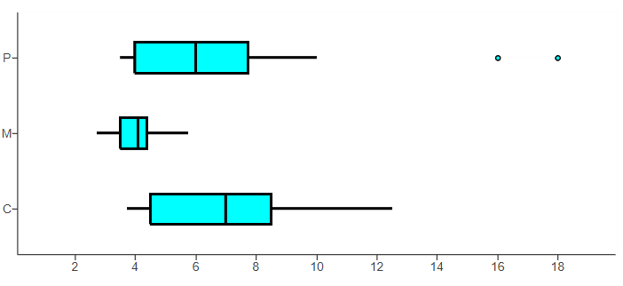
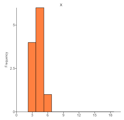
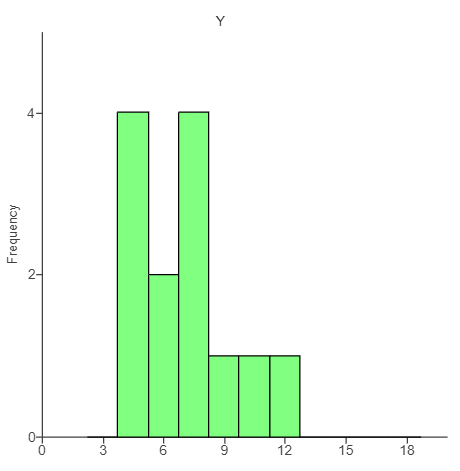
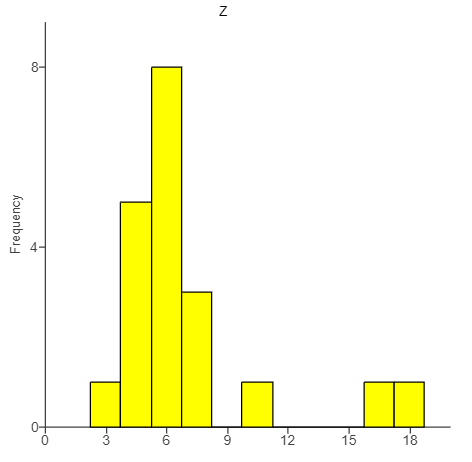
(13.) Three histograms and three boxplots are given below.
Match each histogram (X, Y, and Z) with the corresponding boxplot (A, B, or C).
Explain your reasoning.
Boxplot P corresponds to Histogram Z because both show a right-skewed distribution that has at least
one outlier.
Boxplot M corresponds to Histogram X because both show a symmetric distribution that has no
outliers.
Boxplot C corresponds to Histogram Y because both show a right-skewed distribution that no outliers.
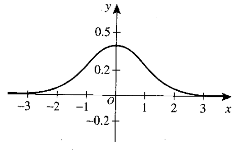
(14.) ACT The standard normal probability distribution function (μ = 0 and σ = 1) is
graphed in the
standard (x, y) coordinate plane below.
Which of the following percentages is closest to the percent of the data points that are within 2
standard deviations of
the mean in any normal distribution?
Empirical Rule: 68 – 95 – 99.7% Rule
Part of the Empirical Rule states that 95% of the data points are within (below and above) 2
standard
deviations from the mean.
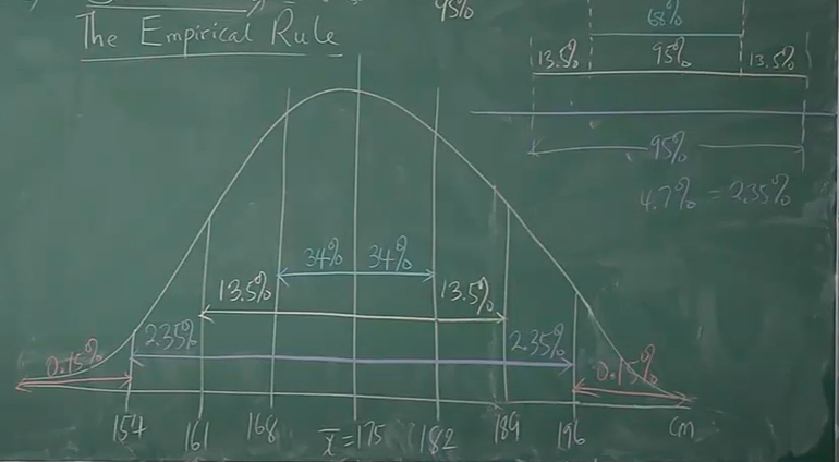
(15.) Assume the heights of the Golden State Warriors basketball team players have a bell-shaped
distribution with mean of 175 cm and
standard deviation of 7 cm.
(a.) Analyze this information using the Empirical Rule.
(b.) (i) Draw the normal distribution curve for the information.
(ii) Indicate the area of each region in the curve.
Treat the dataset as a sample
But you may choose to treat it as a population if you wish
(a.) Empirical Rule: 68 - 95 - 99.7% Rule
$
\bar{x} = 175\;cm \\[3ex]
s = 7\;cm \\[3ex]
1s = 1(7) = 7\;cm \\[3ex]
2s = 2(7) = 14\;cm \\[3ex]
3s = 3(7) = 21\; cm \\[3ex]
\underline{1\;standard\;\;deviation\;\;below\;\;the\;\;mean} \\[3ex]
\bar{x} - 1s \\[3ex]
175 - 7 \\[3ex]
168\;cm \\[3ex]
\underline{1\;standard\;\;deviation\;\;above\;\;the\;\;mean} \\[3ex]
\bar{x} + 1s \\[3ex]
175 + 7 \\[3ex]
182\;cm \\[3ex]
$
This impies that 68% of the basketball team players have heights between 168 cm and 182 cm
$
\underline{2\;standard\;\;deviations\;\;below\;\;the\;\;mean} \\[3ex]
\bar{x} - 2s \\[3ex]
175 - 14 \\[3ex]
161\;cm \\[3ex]
\underline{2\;standard\;\;deviations\;\;above\;\;the\;\;mean} \\[3ex]
\bar{x} + 2s \\[3ex]
175 + 14 \\[3ex]
189\;cm \\[3ex]
$
This impies that 95% of the basketball team players have heights between 161 cm and 189 cm
$
\underline{3\;standard\;\;deviations\;\;below\;\;the\;\;mean} \\[3ex]
\bar{x} - 3s \\[3ex]
175 - 21 \\[3ex]
154\;cm \\[3ex]
\underline{3\;standard\;\;deviations\;\;above\;\;the\;\;mean} \\[3ex]
\bar{x} + 3s \\[3ex]
175 + 21 \\[3ex]
196\;cm \\[3ex]
$
This impies that 99.7% of the basketball team players have heights between 154 cm and 196 cm
(16.) Assume that men's heights have a distribution that is symmetrical and unimodal, with a mean of
62 inches and a standard deviation of 2.5 inches.
(a.) What men's height corresponds to a z-score of 1.20?
(b.) What men's height corresponds to a z-score of −1.20?
$
\mu = 62\;in \\[3ex]
\sigma = 2.5\;in \\[3ex]
(a.) \\[3ex]
z = 1.2 \\[3ex]
x = z\sigma + \mu \\[3ex]
x = 1.2(2.5) + 62 \\[3ex]
x = 65\;inches \\[3ex]
(b.) \\[3ex]
z = -1.2 \\[3ex]
x = z\sigma + \mu \\[3ex]
x = -1.2(2.5) + 62 \\[3ex]
x = 59\;inches
$
(17.)
(18.) Distributions of gestation periods (lengths of pregnancy) for a particular animal are roughly
bell-shaped.
The mean gestation period for this animal is 270 days, and the standard deviation is 5 days for females
who go into spontaneous labor.
Which is more unusual, a baby being born 5 days early or a baby being born 5 days late? Explain.
$
\mu = 270\;days \\[3ex]
\sigma = 5\;days \\[3ex]
z = \dfrac{x - \mu}{\sigma} \\[5ex]
\underline{5\;days\;\;early} \\[3ex]
x = 270 - 5 = 265\;days \\[3ex]
z = \dfrac{265 - 270}{5} \\[5ex]
z = \dfrac{-5}{5} \\[5ex]
z = -1 \\[3ex]
\underline{5\;days\;\;late} \\[3ex]
x = 270 + 5 = 275\;days \\[3ex]
z = \dfrac{275 - 270}{5} \\[5ex]
z = \dfrac{5}{5} \\[5ex]
z = 1 \\[3ex]
$
Both z-scores are within usual values
Both z-scores are the same.
Both events are equally likely.
(19.)
(20.) HSC Mathematics Standard 2 In a particular country, the birth weight of babies is normally
distributed with a mean
of 3000 grams.
It is known that 95% of these babies have a birth weight between 1600 grams and 4400 grams.
One of these babies has a birth weight of 3497 grams.
What is the z-score of this baby's birth weight?
Empirical Rule: 68 - 95 - 99.7% Rule
Part of the Empirical Rule states that 95% of these babies have a birth weight within (below and
above) 2 standard
deviations from the mean
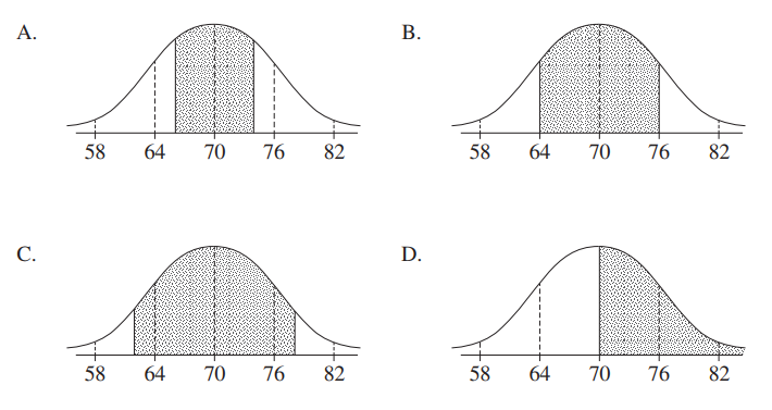
(21.) HSC Mathematics Standard 2 The scores on an examination are normally distributed with a
mean of 70 and a
standard deviation of 6
Michael received a score on the examination between the lower quartile and the upper quartile of the
scores.
Which shaded region most accurately represents where Michael's score lies?
Empirical Rule: 68 - 95 - 99.7% Rule
Part of the Empirical Rule states that 68% of the adult male tibia bones have lengths within (below
and above) 1
standard
deviations from the mean
$
\mu = 70 \\[3ex]
\sigma = 6 \\[3ex]
1s = 1(6) = 6 \\[3ex]
\underline{1\;standard\;\;deviation\;\;below\;\;the\;\;mean} \\[3ex]
\mu - 1\sigma \\[3ex]
70 - 6 \\[3ex]
64 \\[3ex]
\underline{1\;standard\;\;deviation\;\;above\;\;the\;\;mean} \\[3ex]
\mu + 1\sigma \\[3ex]
70 + 6 \\[3ex]
76 \\[3ex]
$
This impies that 68% of the examination scores are between 64 and 76
That means that: 34% of the scores are between 64 and 70
Similarly, 34% of the scores are between 70 and 76
But Option B is not the correct answer
One of the properties of the normal curve is that:
the mean, median, and mode of a normal curve is the same.
This implies that the median is also 70
median = 70 = 50% of the scores
lower quartile = 25% of the scores = 25% below the median
25% is less than 34%
This implies that 25% below the median is less than 64
upper quartile = 75% of the scores = 25% above the median
Similarly, 25% is less than 34%
This implies that 25% above the median is less than 76
So, we are looking for the curve whose shaded area is less than 64 (from the center to the left) and
is also less
than
76 (from the center to the right)
This is because 25% is less than 34% (from the center to the left) and 25% is less than 34% (from
the center to the
right)
This implies that the correct answer is Option A
(22.) Babies born weighing 2500 grams (about 5.5 pounds) or less are called low-birth-weight babies,
and this condition sometimes indicates health problems for the infant.
The mean birth weight for children born in a certain country is about 3417 grams (about 7.5 pounds).
The mean birth weight for babies born one month early is 2604 grams.
Suppose both standard deviations are 460 grams.
Also assume that the distribution of birth weights is roughly unimodal and symmetric.
(a.) Find the standardized score (z-score), relative to all births in the country, for a baby with a
birth weight of 2500 grams.
(b.) Find the standardized score for a birth weight of 2500 grams for a child born one month early,
using 2604 as the mean.
(c.) For which group is a birth weight of 2500 grams more common?
Explain what that implies. Unusual z-scores are far from 0.
$
z = \dfrac{x - \mu}{\sigma} \\[5ex]
\underline{Born\;\;in\;\;a\;\;certain\;\;country} \\[3ex]
\mu = 3417\;grams \\[3ex]
\sigma = 460\;grams \\[3ex]
(a.) \\[3ex]
x = 2500\;grams \\[3ex]
z = \dfrac{2500 - 3417}{460} \\[5ex]
z = -1.993478261 \\[3ex]
z \approx -1.99 \\[5ex]
(b.) \\[3ex]
\underline{Born\;\;one\;\;month\;\;early} \\[3ex]
\mu = 2604\;grams \\[3ex]
\sigma = 460\;grams \\[3ex]
x = 2500\;grams \\[3ex]
z = \dfrac{2500 - 2604}{460} \\[5ex]
z = -0.2260869565 \\[3ex]
z \approx -0.23 \\[3ex]
$
(c.) −0.23 is closer to 0 than −1.99
A birth weight of 2500 grams is more common for babies born one month early.
This makes sense because babies gain weight during gestation, and babies born one month early had
less time to gain weight.
(23.)
(24.) An IQ test has a mean of 103 and a standard deviation of 5.
Which is more unusual, an IQ of 108 or an IQ of 95?
$
z = \dfrac{x - \mu}{\sigma} \\[5ex]
\mu = 103 \\[3ex]
\sigma = 5 \\[3ex]
1st:\;\;x = 108 \\[3ex]
z = \dfrac{108 - 103}{5} \\[5ex]
z = 1 \\[3ex]
z = 1.00 \\[3ex]
2nd:\;\;x = 95 \\[3ex]
z = \dfrac{95 - 103}{5} \\[5ex]
z = -1.6 \\[3ex]
z = -1.60 \\[3ex]
$
1.00 and −1.60 are within usual values.
However, −160 is further from 0 than 1.00.
An IQ of 95 is more unusual because its corresponding z-score, −1.6 is further from 0 than
the corresponding z-score of 1 for an IQ of 108.
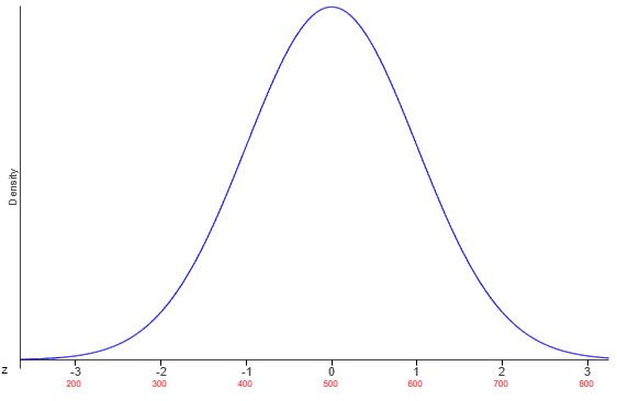
(25.) The quantitative scores on a test are approximately normally distributed with a mean of 500 and a
standard deviation of 100.
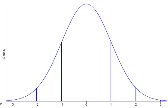
On the horizontal axis of the graph, indicate the test scores that correspond with the provided
z-scores.
Answer the questions using only your knowledge of the Empirical rule and symmetry.
(a.) Indicate the test scores that correspond with the provided z-scores.
(b.) Roughly what percentage of students earn quantitative test scores more than 500?
(c.) Roughly what percentage of students earn quantitative test scores between 400 and 600?
(d.) Roughly what percentage of students earn quantitative test scores more than 800?
(e.) Roughly what percentage of students earn quantitative test scores less than 200?
(f.) Roughly what percentage of students earn quantitative test scores between 300 and 700?
(g.) Roughly what percentage of students earn quantitative test scores between 700 and 800?
(b.) Scores more than 500 is every score above the mean
The percentage of students that earn quantitative test scores more than 500 is 50%
(c.) Scores between 400 and 600 are scores within 1 standard deviation from the mean
The percentage of students that earn quantitative test scores between 400 and 600 is 68%
(d.) Scores more than 800 are scores more than 3 standard deviations above the mean
The percentage of students that earn quantitative test scores more than 800 is 0.15%
(e.) Scores less than 200 are scores less than 3 standard deviations below the mean
The percentage of students that earn quantitative test scores less than 200 is 0.15%
(f.) Scores between 300 and 700 are scores within 2 standard deviations from the mean
The percentage of students that earn quantitative test scores between 300 and 700 is 95%
(g.) Scores between 700 and 800 are scores in-between 2 standard deviations above the mean
and 3 standard
deviations above the mean
The percentage of students that earn quantitative test scores between 700 and 800 is 2.35%
(26.) Answer the following questions.
Show all work.
(I.) In 2017 a pollution index was calculated for a sample of cities in the eastern states using data on
air and water pollution.
Assume the distribution of pollution indices is unimodal and symmetric.
The mean of the distribution was 45.9 points with a standard deviation of 11.3 points.
(a.) What percentage of eastern cities would you expect to have a pollution index between 23.3 and 68.5
points?
(b.) What percentage of eastern cities would you expect to have a pollution index between 34.6 and 57.2
points?
(c.) The pollution index for an eastern city, in 2017, was 56.1 points.
Based on this distribution, was this unusually high? Explain.
(II.) In 2011, the mean property crime rate (per 100,000 people) for 10 northeastern regions of a
certain country was 2416.
The standard deviation was 396.
Assume the distribution of crime rates is unimodal and symmetric.
(a.) What percentage of northeastern regions would you expect to have property crime rates between 2020
and 2812?
(b.) What percentage of northeastern regions would you expect to have property crime rates between 1624
and 3208?
(c.) If someone guessed that the property crime rate in one northeastern region was 9004, would this
number be consistent with the data set?
First find the upper bound for three standard deviations from the mean.
Is 9004 consistent with the data set?
(I.)
$
\bar(x) = 45.9\;points \\[3ex]
s = 11.3\;points \\[3ex]
(a.) \\[3ex]
1\;standard\;\;deviation\;\;from\;\;the\;\;mean \\[3ex]
\bar{x} - s \\[3ex]
45.9 - 11.3 = 34.6 \\[3ex]
\bar{x} + s \\[3ex]
45.9 + 11.3 = 57.2 \\[3ex]
2\;standard\;\;deviations\;\;from\;\;the\;\;mean \\[3ex]
\bar{x} - 2s \\[3ex]
45.9 - 2(11.3) = 23.3 \\[3ex]
\bar{x} + 2s \\[3ex]
45.9 + 11.3 = 68.5 \\[3ex]
$
95% of eastern cities are expected to have a pollution index between 23.3 and 68.5 points
68% of eastern cities are expected to have a pollution index between 34.6 and 57.2 points
(c.) No, because 56.1 falls within two standard deviations away from the mean, and it is therefore
not an unusually high pollution index.
(II.)
$
\bar(x) = 2416 \\[3ex]
s = 396 \\[3ex]
(a.) \\[3ex]
1\;standard\;\;deviation\;\;from\;\;the\;\;mean \\[3ex]
\bar{x} - s \\[3ex]
2416 - 396 = 2020 \\[3ex]
\bar{x} + s \\[3ex]
2416 + 396 = 2812 \\[3ex]
$
The percentage of northeastern regions expected to have property crime rates between 2020 and 2812
is 68%
$
2\;standard\;\;deviations\;\;from\;\;the\;\;mean \\[3ex]
\bar{x} - 2s \\[3ex]
2416 - 2(396) = 1624 \\[3ex]
\bar{x} + 2s \\[3ex]
2416 + 2(396) = 3208 \\[3ex]
$
The percentage of northeastern regions expected to have property crime rates between 1624 and 3208
is 95%
$
(c.) \\[3ex]
3\;standard\;\;deviations\;\;from\;\;the\;\;mean \\[3ex]
\bar{x} - 3s \\[3ex]
Lower\;\;bound= 2416 - 3(396) = 1228 \\[3ex]
\bar{x} + 3s \\[3ex]
Upper\;\;bound = 2416 + 3(396) = 3604 \\[3ex]
$
Is 9004 consistent with the data set?
No, because 9004 falls well above three standard deviations away from the mean, and it is therefore
unlikely that a region would have this value.
(27.)
(28.)
(29.)
(30.)
(31.)
(32.)
(33.)
(34.)
(35.)
(36.)
(37.)
(38.)
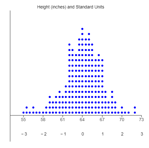
(39.) The dotplot shows heights of college women; the mean is 64 inches (5 feet 4 inches) and the
standard deviation is 3 inches.
(a.) What is the z-score for a height of 67 inches (5 feet 7 inches)?
(b.) What is the height of a woman with a z-score of −2?
We can solve this question in at least two ways
Use any approach you prefer.
Based on the dotplot:
(a.) The z-score for a height of 67 inches = 1
(b.) The height of a woman with a z-score of −2 = 58 inches
Based on Calculations:
$
z = \dfrac{x - \mu}{\sigma} \\[5ex]
\mu = 64\;inches \\[3ex]
\sigma = 3\;inches \\[3ex]
(a.) \\[3ex]
x = 67\;inches \\[3ex]
z = \dfrac{67 - 64}{3} \\[5ex]
z = 1 \\[3ex]
(b.) z = -2 \\[3ex]
x = z\sigma + \mu \\[3ex]
x = -2(3) + 64 \\[3ex]
x = 58\;inches
$
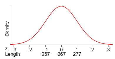
(59.) Assume that the lengths of pregnancy for humans are approximately normally distributed, with a
mean of 267 days and a standard deviation of 10 days.
Use the Empirical Rule to answer the following questions.
Do not use the technology or the Normal table.
Begin by labeling the horizontal axis of the graph with lengths, using the given mean and standard
deviation.
(a.) Roughly what percentage of pregnancies last more than 267 days?
(b.) Roughly what percentage of pregnancies last between 267 and 277 days?
(c.) Roughly what percentage of pregnancies last less than 237 days?
(d.) Roughly what percentage of pregnancies last between 247 and 287 days?
(e.) Roughly what percentage of pregnancies last longer than 287 days?
(f.) Roughly what percentage of pregnancies last longer than 297 days?
Based on the Empirical Rule and the Empirical Rule Table above:
(b.) Between 267 and 277 is 1 standard deviation above the mean
The percentage of pregnancies that last between 267 and 277 days is 34%
(c.) Less than 237 days is less than 3 standard deviations below the mean
The percentage of pregnancies that last less than 237 days is 0.15%
(d.) Between 247 and 287 is 2 standard deviations above the mean
The percentage of pregnancies that last between 247 and 287 days is 95%
(e.) Longer than 287 days is more than 2 standard deviations above the mean
The percentage of pregnancies that last longer than 287 days is 2.35% + 0.15% = 2.5%
(f.) Longer than 297 days is more than 3 standard deviations above the mean
The percentage of pregnancies that last longer than 287 days is 0.15%
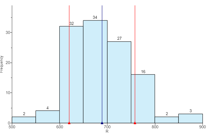
(61.) The accompanying histogram shows the number of runs scored by baseball teams for three seasons.
The distribution is roughly unimodal and symmetric, with a mean of 689 and a standard deviation of 69
runs.
An interval one standard deviation above and below the mean is marked on the histogram. Assume the
values in a bin are distributed uniformly.
For example, if the leftmost line is at the midpoint, then half of that bin's values are below the
line and half are above.
(a.) According to the Empirical Rule, approximately what percent of the data should fall in the
interval from 620 to 758 (that is, one standard deviation above and below the mean)?
(b.) Use the histogram to estimate the actual percent of teams that fall in this interval.
How did your estimate compare to the value predicted by the Empirical Rule?
(c.) Between what two values would you expect to find about 95% of the teams?
(a.) Approximately 68% of the data should fall in the interval from 620 to 758.
(b.) 69% of the data falls in the interval from 620 to 758.
The estimate is very close to the value predicted by the Empirical Rule.
$
(c.) \\[3ex]
\underline{Empirical\;\;Rule} \\[3ex]
\bar{x} = 689\;runs \\[3ex]
s = 69\;runs \\[3ex]
\bar{x} - 2s \\[3ex]
= 689 - 2(69) \\[3ex]
= 689 - 138 \\[3ex]
= 551 \\[3ex]
\bar{x} + 2s \\[3ex]
= 689 + 2(69) \\[3ex]
= 689 + 138 \\[3ex]
= 827 \\[3ex]
$
You expect to find about 95% of the teams between the two values 551 and 827.